6. Examples

6.1. Measuring stellar radial velocities

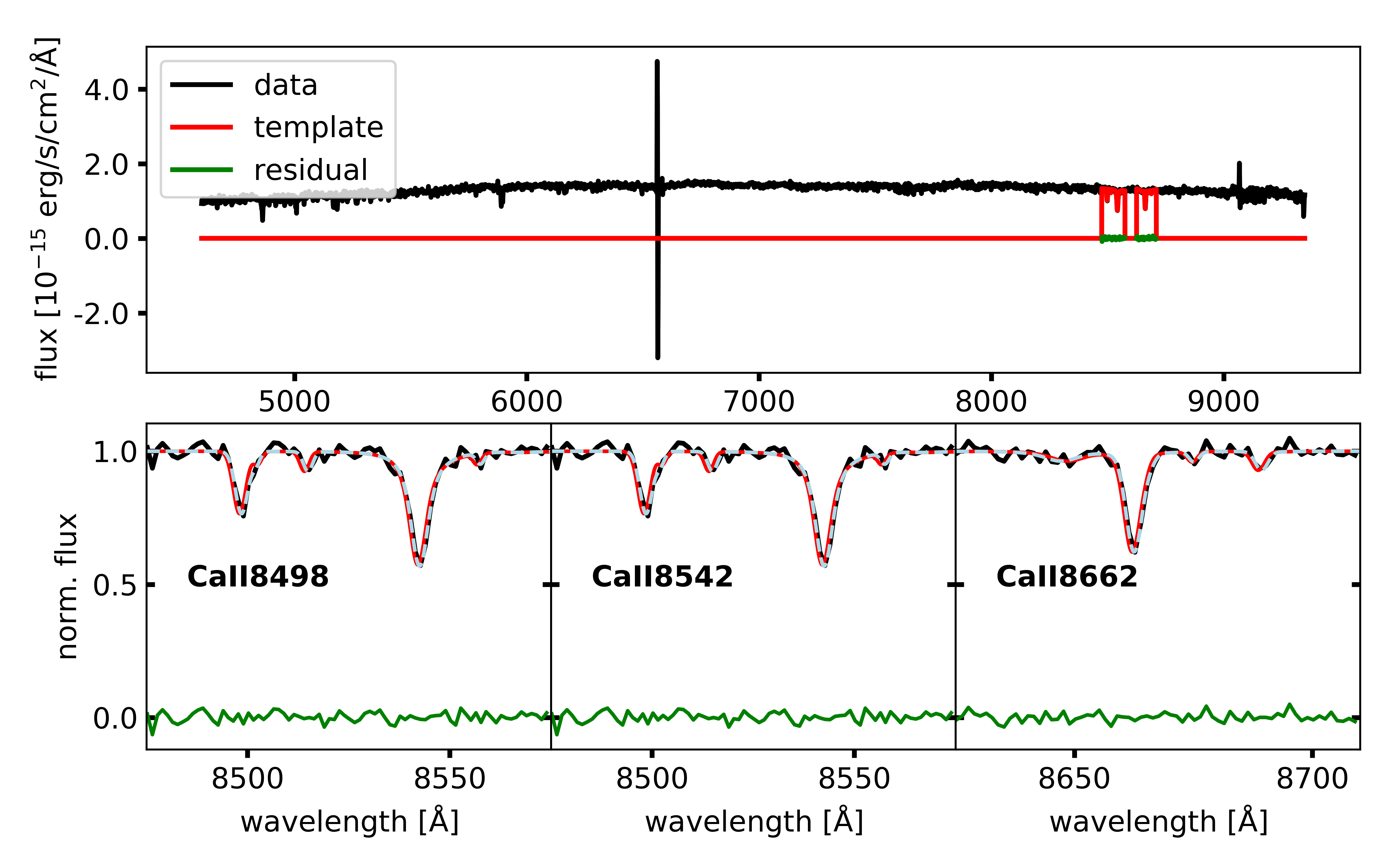
In this tutorial we show the user how to create a spectral measure the stellar radial velocity. All files in including the example code may be downloaded by using the individual links or as a zip-archive here. The stellar spectrum used in this example contains the PampelMuse extracted spectrum of a member pre-main-sequence member star of the young massive star cluster Westerlund 2 showing a pronounced CaII-Triplet, which we will use to measure the RV. The user can also see that the Balmer lines are not well extracted, which is caused by the high nebular emission lines (Zeidler et al. 2018, Zeidler et al. 2019) demonstrating that this does not influence the radial velocity fit.

6.1.1. The procedure

1. Reading in the necessary data

   As a first step we must read the necessary data. This includes the spectrum, the spectral line library, and the line list of the spectral lines that are used to measure the radial velocity. Since the CaII-Triplet lines are blended with the Paschen Series, we also have to include a catalog of the blends.

   from astropy.io import ascii
   from astropy.io import fits
   import numpy as np
   from MUSEpack.radial_velocities import RV_spectrum
   
   spec_hdu = fits.open('star.fits')
   lcat = ascii.read('line_library.dat')['wavelength']
   blends = 'blends.dat'
   target_lines = 'target_lines.list'
   

2. Creating the flux, flux uncertainty, and wavelength arrays, as well as the line lists In this step all the necessary arrays are created from the input files. The header information of the stellar spectrum is used to create the wavelength array. The flux is stored in the first extension while the flux uncertainties are stored in the second extension of the stellar spectrum.

   Note

   The MUSE fluxes are stored in \(10^{20}\,{\rm erg}\,{\rm s}^{-1}\,{\rm cm}^{-2}\,{\rm A}^{-1}\). Therefore, we need to multiply the flux and uncertainty array with \(10^{-20}\)

   spec_head = spec_hdu[0].header
   spec_wave = np.arange(spec_head['NAXIS1']) * spec_head['CDELT1'] + spec_head['CRVAL1']
   spec_data = spec_hdu[0].data * 10e-20
   spec_error = spec_hdu[1].data * 10e-20
   

3. We are now initiating the spectral instance. The ID of the star will be star_1. We initiate the instance in INFO mode.

   spfit = RV_spectrum('star_1', spec_data, spec_error, spec_wave, loglevel='INFO')
   

4. As next step we need to initiate the catalog populated with the absorption lines, with which we want to measure the radial velocity. This catalog will contain all the fitted parameters and may be called at any point calling spfit.cat

   spfit.catalog(initcat=target_lines)
   

At this point the spectral instance is fully initiated and we can start working with it.

5. We now run the spectral fit using all available cores. The line indices may be read directly from the instance’s catalog. A log file named star_1.log will be automatically created

   spfit.line_fitting(lcat, spfit.cat.index, resid_level=0.05,\
   max_contorder=2, niter=10, adjust_preference='contorder', n_CPU=-1,\
   max_ladjust=2, max_exclusion_level=0.3, blends=blends,\
   llimits=[-2., 2.], autoadjust=True, fwhm_block=True,\
   input_continuum_deviation=0.05)
   

6. We will now plot the fitted spectrum to a file called star_1_plot.png. The fitted spectrum will be oversampled.

   spfit.plot(oversampled=True)
   

At this point the spectral instance contains the spectrum as well as the fitted template. The next steps will execute the radial velocity determination.

7. First we determine the radial velocity purely based on the line peaks. The measured peak velocity and its uncertainty may be called at any time using spfit.rv_peak and spfit.erv_peak, respectively.

   spfit.rv_fit_peak(line_sigma=3, line_significants=5)
   

8. Now we measure the radial velocities using the Monte Carlo bootstrap method. As initial guess we use the peak velocity spfit.rv_peak. We sample the spectrum 20000 times and use all available CPUs. The measured radial velocity and its uncertainty may be called at any time using spfit.rv and spfit.erv, respectively.

   spfit.rv_fit([spfit.rv_peak, 0.], niter=20000, n_CPU=-1)
   

9. The measured radial velocities (per line and for the star) are added to the spectral instance. We may now write the fitted parameters to an ASCII file. Additionally we may print the radial velocity of the star measure with the peaks only and with the the full spectrum.

   spfit.catalog(save=True, printcat=True)
   

6.1.2. The results

After successfully executing the script the radial velocity of star_1 is \(13.90 \pm 1.949\,{\rm km}\,{\rm s}^{-1}\) based on two out of the three absorption lines. The radial velocity based on the peaks only is \(15.43 \pm 1.144\,{\rm km}\,{\rm s}^{-1}\) and agrees well with the cross correlation.

Note

The user should keep in mind that the radial velocity fit is a statistical Monte Carlo process so the final result may fluctuate slightly. All tests showed that these fluctuations are magnitudes smaller than the intrinsic uncertainty caused by a the limited spectral resolution and S/N.

The final results for each individual line, also documented in the star_1.cat file, are the following:

	l_lab	l_start	l_end	l_fit	a_fit	sg_fit	sl_fit	cont_order	RV	eRV	used	significance
CaII8498	8498.02	8475.0	8575.0	8498.528526	-3.17e-16	1.59	0.00	2	19.67	3.797		17.628082
CaII8542	8542.09	8475.0	8575.0	8542.529694	-1.14e-15	1.29	1.63	2	14.58	2.395	x	63.591358
CaII8662	8662.14	8625.0	8710.0	8662.552815	-5.64e-16	1.58	0.33	2	13.84	2.709	x	30.051289

The CaII8498 lines was discarded because it did not fulfill the \(3\sigma\) criterion. The user may loosen the line_sigma parameter in the radial_velocities.RV_spectrum.rv_fit module to adjust the exclusion limits.

The following figure shows the line fit printed to star_1_plot.png

6.2. Additional tutorials

Todo

We will add more tutorials in the near future…